CU Mechanical Engineering Fluid Mechanics Matlab tutorials

---

Writing Matlab Functions: modeling the spread of disease

In this example, we will write a function that models the spread of infectious diseases.

global a b
a = 0;
b= 0;

In the beginning of this script, we define some of the variables we are going to use. The 'global' command defines global variables. Ordinarily, each MATLAB function, defined by an M-file, has its own local variables, which are separate from those of other functions, and from those of the base workspace. However, if several functions, and possibly the base workspace, all declare a particular name as global, they all share a single copy of that variable. Any assignment to that variable, in any function, is available to all the functions declaring it global.

Now to set up the model we input the following:

for cs =1:3
    if cs == 1
        a=1e-5;
        b=0.25;
        ttle='Case a: no spread of disease';
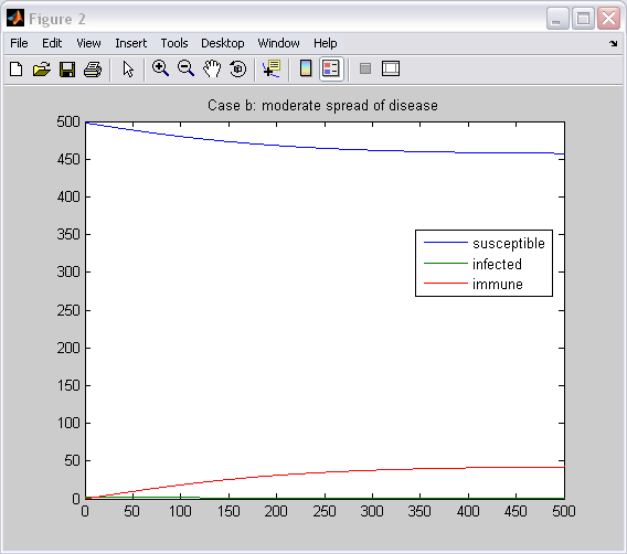
    elseif cs == 2
        a=2e-4;
        b=0.1;
        ttle='Case b: moderate spread of disease';
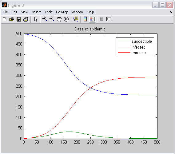
    elseif cs == 3
        a=1.5e-4;
        b=0.05;
        ttle='Case c: epidemic'
    end
    tspan=[0:1:730];
    options = odeset('RelTol',1e-12,'AbsTol',1e-6,'NormControl','on','MaxOrder',2);
    [T,Y] = ode15s(@fun_cp5,tspan,[498 2 0],options);
    figure(cs)
    hold off
    plot(T,Y(:,1:3))
    legend('susceptible','infected','immune',0)
    title(ttle)
    set(gca,'xlim',[0 500])
end

We begin by defining three different sets of initial conditions for the ordinary differential equation. This is easily accomplished with one instance of a 'for' loop coupled with a conditional 'if' statement. The time interval for the set is defined in a vector. The odeset function lets you adjust the integration parameters of the ODE solvers. 'options = odeset('name1',value1,'name2',value2,...)' creates an options structure that you can pass as an argument to any of the ODE solvers. In the resulting structure, options, the named properties have the specified values. For example, 'name1' has the value 'value1'. Any unspecified properties have default values. A variable order solver based on the numerical differentiation formulas (NDFs), ode15s optionally uses the backward differentiation formulas, BDFs (also known as Gear's method). Like ode113, ode15s is a multistep solver. It should be noted that the '@' sign means right before 'fun_cp5' means that 'fun_cp5' is a function, not a variable. We'll define the fun_cp5 function as follows:

function dy = fun_cp5(t,y)

The differentail equations we are modeling with this function are:

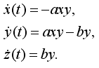
We will define these equations in the fun_cp5function as follows:

global a b;
dy = zeros(3,1);    
dy(1) = -a * y(1) * y(2);
dy(2) = a * y(1) * y(2) - b * y(2);
dy(3) = b * y(2);

Returning to the 'disease' function, the last block of code sets the plot properties.

The m-file can now be saved as 'disease.m' The following is a sample output from the code illustrating the way to call the function with the return arguments.

>> disease

ttle =

Case c: epidemic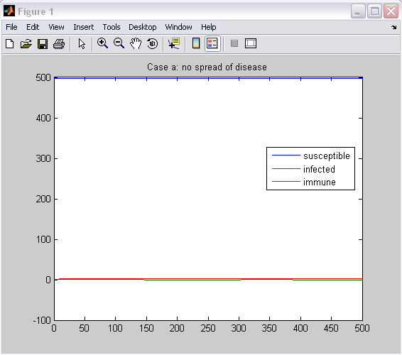

The entire matlab script can be seen below or downloaded here (right-click to save):

global a b
a = 0;
b= 0;

for cs =1:3
    if cs == 1
        a=1e-5;
        b=0.25;
        ttle='Case a: no spread of disease';
    elseif cs == 2
        a=2e-4;
        b=0.1;
        ttle='Case b: moderate spread of disease';
    elseif cs == 3
        a=1.5e-4;
        b=0.05;
        ttle='Case c: epidemic'
    end
    tspan=[0:1:730];
    options = odeset('RelTol',1e-12,'AbsTol',1e-6,'NormControl','on','MaxOrder',2);
    [T,Y] = ode15s(@fun_cp5,tspan,[498 2 0],options);
    figure(cs)
    hold off
    plot(T,Y(:,1:3))
    legend('susceptible','infected','immune',0)
    title(ttle)
    set(gca,'xlim',[0 500])
end

%----------------------------------------

%fun_cp5

function dy = fun_cp5(t,y)
global a b;
dy = zeros(3,1);  
dy(1) = -a * y(1) * y(2);
dy(2) = a * y(1) * y(2) - b * y(2);
dy(3) = b * y(2);

---