CU Mechanical EngineeringFluid Mechanics Matlab tutorials |
Writing Matlab Functions: integration with different parameters
In this example, we will write a function that integrates the equation
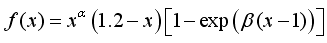
using the trapezoidal rule, Simpson’s rule, and adaptive quadrature algorithm based on the trapezoidal rule.
To begin, all functions within matlab must begin by declaring that m-file is a function. This is accomplished by having the first line of the m-file having the word 'function' followed by the name of the variable that will be returned. This is consequently set equal to the name of the name of the file with the quantities that are passed to the function in parenthesis. For the purpose of this exercise, the name of the function will be 'cp4' and the first lines of the function is as follows:
function cp4
global isub
syms f t
close all
figure(1)
After naming the function, we define the global variable 'isub'. Ordinarily, each MATLAB function, defined by an M-file, has its own local variables, which are separate from those of other functions, and from those of the base workspace. However, if several functions, and possibly the base workspace, all declare a particular name as global, they all share a single copy of that variable. Any assignment to that variable, in any function, is available to all the functions declaring it global. The line 'syms f t' is short-hand notation for:
f = sym('f');
t = sym('t'); ...
'close all' deletes all figures whose handles are not hidden. figure(1) does one of two things, depending on whether or not a figure with handle 1 exists. If 1 is the handle to an existing figure, figure(1) makes the figure identified by 1 the current figure, makes it visible, and raises it above all other figures on the screen. The current figure is the target for graphics output. If 1 is not the handle to an existing figure, but is an integer, figure(1) creates a figure and assigns it the handle 1. figure(1) where 1 is not the handle to a figure, and is not an integer, is an error.
The following sets up the initial conditions for both cases:
for cs = 1:2
    if cs ==1
        alpha = 2;
        beta = 0.2;
        I_ex= 0.0095499658265276;
        f = t^alpha*(6/5-t)*(1-exp(beta*(t-1)));
        subplot(2,2,1)
    elseif cs == 2
        alpha = 0.2;
        beta = 2;
        I_ex= 0.3457273592825;
        f = t^alpha*(6/5-t)*(1-exp(beta*(t-1)));
        subplot(2,2,2)
    end
The next step is block of code it as follows:
    xvec=linspace(0,1,101);
    fvec=subs(f,xvec);
    plot(xvec,fvec,'r-');
    grid on
    if cs == 1
        del=[1.e-1,1.e-2,1.e-3,1.e-4,1.e-5,1.e-6,1.e-7,1.e-8,1.e-9,1.e-10,1.e-11] ;
        n=[20,40,80,160,320,640,1280];
        ttl='Case a';
    else
        del=[1.e-1,1.e-2,1.e-3,1.e-4,1.e-5,1.e-6,1.e-7,1.e-8] ;
        n=[20,40,80,160,320,640,1280,2560,5120,10240];
        ttl='Case b';
    end
The linspace function generates linearly spaced vectors. It is similar to the colon operator ":", but gives direct control over the number of points. 'y = linspace(a,b,n)' generates a row vector 'y' of n points linearly spaced between and including a and b. In the next line of code, subs(f,xvec) replaces the default symbolic variable in f with xvec. 'grid on' adds major grid lines to the current axes. The following conditional 'if' statement defines the array of intervals and tolerances.
The next few lines of code create arrays of all zeros.
    err_Simpson=zeros(size(n));
    n_adapt=zeros(size(del));
    err_adapt=zeros(size(del));
    title(ttl);
    disp(ttl);
The command 'B = zeros(size(A))' returns an array the same size as A consisting of all zeros.
Next we have to integrate. For this step, we need two other functions: one using the adaptive quadrature algorithm based on the trapezoidal rule and the other using Simpson’s rule. First we'll create the function integrate_Simpson:
function I=integrate_Simpson(f,a,b,n)
xvec=linspace(a,b,n+1);
fvec=subs(f,xvec);
h = (b-a)/n;
I=h/3*(fvec(1)+4*sum(fvec(2:2:n))+2*sum(fvec(3:2:n-1))+fvec(n+1));
To begin, as with all functions within matlab, it must begin by declaring that the m-file is a function. This is accomplished by having the first line of this m-file having the word 'function' followed by the name of the variable that will be returned. This is consequently set equal to the name of the name of the file with the quantities that are passed to the function in parenthesis. Within the parenthesis are the defining parameters, which are: f, which is the symbolically defined function of one variable; a, the lower limit of integration; b, the upper limit of integreation; and n, the number of subintercals. The fourth line of this function, 'h = (b-a)/n', describes the grid spacing. The last line is the integral itself.
Next we create the function adaptive_quadrature:
function I = adaptive_quadrature(f,a,b,delta)
global isub
I2=integrate_Simpson(f,a,b,2);
I4=integrate_Simpson(f,a,b,4);
err=abs(I2-I4)/15;
isub = isub + 1;
if err < delta
    I=I4;
else
    I=adaptive_quadrature(f,a,(a+b)/2,delta/2)+adaptive_quadrature(f,(a+b)/2,b,delta/2);
end
Again, we begin by having the first line of this m-file having the word 'function' followed by the name of the variable that will be returned. This is consequently set equal to the name of the name of the file with the quantities that are passed to the function in parenthesis. Within the parenthesis are the defining parameters, which are: f, which is the symbolically defined function of one variable; a, the lower limit of integration; b, the upper limit of integreation; and delta, which corresponds to the desired tolerance. The second line defines 'isub' as a global variable. In the next line, we use Simpson's integration rule over interval [a,b] using 3 points, and the next line uses Simpson's integration rule over interval [a,b] using 5 points. The next line, 'err=abs(I2-I4)/15' is the error estimate. Line six calculates the number of times the quadrature is called. The conditional 'if' statement tells the function to stop if the error is below the desired tolerance, and otherwise to refine the interval and call the same function again.
Back to the fucntion cp4, we can now put these functions to use:
    for i=1:length(n)
        disp(['Simpson integration with ',num2str(n(i)),' points']);
        I_Simpson=integrate_Simpson(f,0,1,n(i));
        err_Simpson(i)=abs(I_Simpson-I_ex);
    end
    for i=1:length(del)
        isub = 1;
        disp(['Adaptive quadrature with ',num2str(del(i)),' tolerance']);
        I_adapt=adaptive_quadrature(f,0,1,del(i));
        err_adapt(i)=abs(I_adapt-I_ex);
        n_adapt(i)=2*isub;
    end
This block of code evaluates the external functions. The command 'disp(X)' displays an array, without printing the array name. If X contains a text string, the string is displayed.
To finish the function and obtain the desired plots, we input the following:
    if cs == 1
        subplot(2,2,3)
    elseif cs == 2
        subplot(2,2,4)
    end
    loglog(n,err_Simpson,'r-')
    grid on
    set(gca,'xlim',[10,1e4],'XMinorGrid','off','YMinorGrid','off')
    set(gca,'xTick',[10 10^2 10^3 10^4 10^5])
    set(gca,'yTick',[1e-16 1e-14 1e-12 1e-10 1e-8 1e-6 1e-4 1e-2 1 10])
    hold on
    plot(n_adapt,err_adapt,'k-')
    legend('Simpson','Ad. Quadr.')
    legend boxon
end
The command subplot divides the current figure into rectangular panes that are numbered rowwise. Each pane contains an axes object. Subsequent plots are output to the current pane. 'h = subplot(m,n,p)' or 'subplot(mnp)' breaks the figure window into an m-by-n matrix of small axes, selects the path axes object for the current plot, and returns the axes handle. The axes are counted along the top row of the figure window, then the second row, etc. Next, 'loglog(X1,Y1,...)' plots all Xn versus Yn pairs. If only Xn or Yn is a matrix, loglog plots the vector argument versus the rows or columns of the matrix, depending on whether the vector's row or column dimension matches the matrix. We already discussed the 'grid on' command. 'set(H,'PropertyName',PropertyValue,...)' sets the named properties to the specified values on the object(s) identified by H. H can be a vector of handles, in which case set sets the properties' values for all the objects. The 'hold' function determines whether new graphics objects are added to the graph or replace objects in the graph. 'hold on' retains the current plot and certain axes properties so that subsequent graphing commands add to the existing graph. 'legend' places a legend on various types of graphs (line plots, bar graphs, pie charts, etc.). For each line plotted, the legend shows a sample of the line type, marker symbol, and color beside the text label you specify. When plotting filled areas (patch or surface objects), the legend contains a sample of the face color next to the text label.
The m-file can now be saved as 'cp4.m' The following are several sample outputs from the code illustrating the ways to call the function with different types of return arguments.
>> cp4
Case a
Simpson integration with 20 points
Simpson integration with 40 points
Simpson integration with 80 points
Simpson integration with 160 points
Simpson integration with 320 points
Simpson integration with 640 points
Simpson integration with 1280 points
Adaptive quadrature with 0.1 tolerance
Adaptive quadrature with 0.01 tolerance
Adaptive quadrature with 0.001 tolerance
Adaptive quadrature with 0.0001 tolerance
Adaptive quadrature with 1e-005 tolerance
Adaptive quadrature with 1e-006 tolerance
Adaptive quadrature with 1e-007 tolerance
Adaptive quadrature with 1e-008 tolerance
Adaptive quadrature with 1e-009 tolerance
Adaptive quadrature with 1e-010 tolerance
Adaptive quadrature with 1e-011 tolerance
Case b
Simpson integration with 20 points
Simpson integration with 40 points
Simpson integration with 80 points
Simpson integration with 160 points
Simpson integration with 320 points
Simpson integration with 640 points
Simpson integration with 1280 points
Simpson integration with 2560 points
Simpson integration with 5120 points
Simpson integration with 10240 points
Adaptive quadrature with 0.1 tolerance
Adaptive quadrature with 0.01 tolerance
Adaptive quadrature with 0.001 tolerance
Adaptive quadrature with 0.0001 tolerance
Adaptive quadrature with 1e-005 tolerance
Adaptive quadrature with 1e-006 tolerance
Adaptive quadrature with 1e-007 tolerance
Adaptive quadrature with 1e-008 tolerance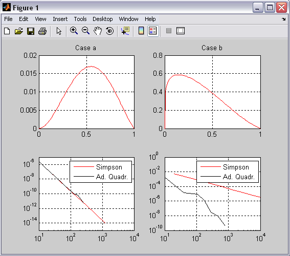
The entire matlab script can be seen below or downloaded here (right-click to save):
function cp4
global isub
syms f t
close all
figure(1)
for cs = 1:2
    if cs ==1
        alpha = 2;
        beta = 0.2;
        I_ex= 0.0095499658265276;
        f = t^alpha*(6/5-t)*(1-exp(beta*(t-1)));
        subplot(2,2,1)
    elseif cs == 2
        alpha = 0.2;
        beta = 2;
        I_ex= 0.3457273592825;
        f = t^alpha*(6/5-t)*(1-exp(beta*(t-1)));
        subplot(2,2,2)
    end
    xvec=linspace(0,1,101);
    fvec=subs(f,xvec);
    plot(xvec,fvec,'r-');
    grid on
    if cs == 1
        del=[1.e-1,1.e-2,1.e-3,1.e-4,1.e-5,1.e-6,1.e-7,1.e-8,1.e-9,1.e-10,1.e-11] ;
        n=[20,40,80,160,320,640,1280];
        ttl='Case a';
    else
        del=[1.e-1,1.e-2,1.e-3,1.e-4,1.e-5,1.e-6,1.e-7,1.e-8] ;
        n=[20,40,80,160,320,640,1280,2560,5120,10240];
        ttl='Case b';
    end
    err_Simpson=zeros(size(n));
    n_adapt=zeros(size(del));
    err_adapt=zeros(size(del));
    title(ttl);
    disp(ttl);
    for i=1:length(n)
        disp(['Simpson integration with ',num2str(n(i)),' points']);
        I_Simpson=integrate_Simpson(f,0,1,n(i));
        err_Simpson(i)=abs(I_Simpson-I_ex);
    end
    for i=1:length(del)
        isub = 1;
        disp(['Adaptive quadrature with ',num2str(del(i)),' tolerance']);
        I_adapt=adaptive_quadrature(f,0,1,del(i));
        err_adapt(i)=abs(I_adapt-I_ex);
        n_adapt(i)=2*isub;
    end

    if cs == 1
        subplot(2,2,3)
    elseif cs == 2
        subplot(2,2,4)
    end
    loglog(n,err_Simpson,'r-')
    grid on
    set(gca,'xlim',[10,1e4],'XMinorGrid','off','YMinorGrid','off')
    set(gca,'xTick',[10 10^2 10^3 10^4 10^5])
    set(gca,'yTick',[1e-16 1e-14 1e-12 1e-10 1e-8 1e-6 1e-4 1e-2 1 10])
    hold on
    plot(n_adapt,err_adapt,'k-')
    legend('Simpson','Ad. Quadr.')
    legend boxon
end

%---------------------------------------------------------

%integrate_Simpson

function I=integrate_Simpson(f,a,b,n)
xvec=linspace(a,b,n+1);
fvec=subs(f,xvec);
h = (b-a)/n;
I=h/3*(fvec(1)+4*sum(fvec(2:2:n))+2*sum(fvec(3:2:n-1))+fvec(n+1));

%------------------------------------------------------

%adaptive_quadrature

function I = adaptive_quadrature(f,a,b,delta)
global isub
I2=integrate_Simpson(f,a,b,2);
I4=integrate_Simpson(f,a,b,4);
err=abs(I2-I4)/15;
isub = isub + 1;
if err < delta
    I=I4;
else
    I=adaptive_quadrature(f,a,(a+b)/2,delta/2)+adaptive_quadrature(f,(a+b)/2,b,delta/2);
end