CU Mechanical EngineeringNumerical Methods Matlab tutorials |
Writing Matlab Functions: polynomial interpolation
In this example, we will write a function that will help us study the effect of the choice of polynomial interpolation points on a given interval.
To begin, all functions within matlab must begin by declaring that m-file is a function. This is accomplished by having the first line of the m-file having the word 'function' followed by the name of the variable that will be returned. This is consequently set equal to the name of the name of the file with the quantities that are passed to the function in parenthesis. For the purpose of this exercise, the name of the function will be 'cp3' and the first line of the function is as follows:
function cp3
This function utilzes nested functions to evaluate the algorithm for several differnt cases. The nested function used will be described momentarily. The rest of this function is as follows:
n=[1,5,10,15];
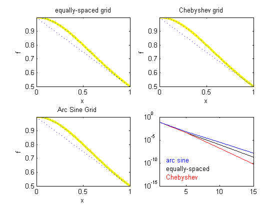
cp3_4figs('1/(1+x^2)',n,0)
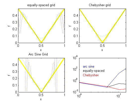
cp3_4figs('abs(x-0.5)',n,1)
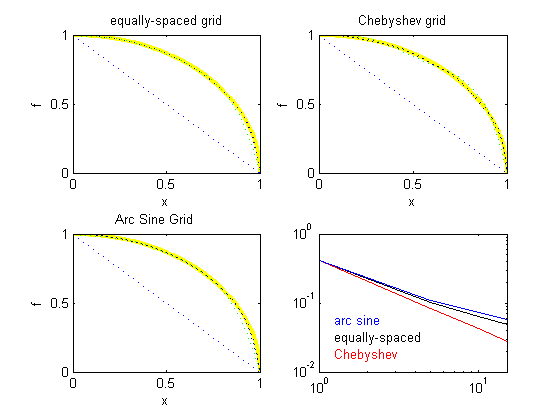
cp3_4figs('sqrt(1-x^2)',n,1)
By defining a separate function to interpolate an input function, multiple functions can easily be evaluated and compared.
The function 'cp3_4figs' takes. The first line of this function is as follows:
function cp3_4figs(f,n,xlog)
This function takes three arguments. The first is the function, the second is the number of points to use for the interpolation and the last is used to determine which kind of plot to use. This will come in to play shortly.
figure
x=linspace(0,1,1001);
f_exact=subs(f,x);
linestyle=['k: ';'b: ';'g: ';'m: '];
titles=['equally-spaced grid';...
        'Chebyshev grid     ';...
        'Arc Sine Grid      '];
The above segment of code sets up the plot. The 'linestyles' command sets the colors for each of the different data sets being plotted. The first letter corresponds to the color and the colon indicates that the line is to be plotted as a dotted line. The 'titles' array identifies the kind of distributions used for the points. This information will be available in the legend.
for i=1:3
    subplot(2,2,i);
    plot(x,f_exact,'y-','linewidth',3);
    xlabel('x');
    ylabel('f');
    title(titles(i,:));
    hold on
end
'subplot' divides the current figure into rectangular panes that are numbered rowwise. Each pane contains an axes object. Subsequent plots are output to the current pane. The 'subplot(2,2,i)' command sets up a 2x2 grid of plots and the 'for' loop goes through and plots in each quadrant.
for i=1:size(n,2)
    i1=mod(i,3)+1;
    k      = linspace(0,n(i),n(i)+1);
    x_eq   = k/n(i);
    x_ch   = (1-cos(pi*k/n(i)))/2;
    x_asin = 0.5+asin(2.*k./n(i)-1)./pi;
    f_eq   = interpolate_mine(x,x_eq  ,subs(f,x_eq  ));
    f_ch   = interpolate_mine(x,x_ch  ,subs(f,x_ch  ));
    f_asin = interpolate_mine(x,x_asin,subs(f,x_asin));
    err(i,1)  = max(abs(f_exact-f_eq  ));
    err(i,2)  = max(abs(f_exact-f_ch  ));
    err(i,3)  = max(abs(f_exact-f_asin));
    subplot(2,2,1);
    plot(x,f_eq,linestyle(i1,:),'linewidth',1);
    set(gca,'ylim',[min(f_exact),max(f_exact)])
    subplot(2,2,2);
    plot(x,f_ch,linestyle(i1,:),'linewidth',1);
    set(gca,'ylim',[min(f_exact),max(f_exact)])
    subplot(2,2,3);
    plot(x,f_asin,linestyle(i1,:),'linewidth',1);
    set(gca,'ylim',[min(f_exact),max(f_exact)])
end
The above segment of begins by calculating the diffent point distributions. The 'linspace' function generates linearly spaced vectors. It is similar to the colon operator ":", but gives direct control over the number of points. One the point distribution have been defined, the function 'interpolate_mine' is called for each of the three different cases. This function is explained in more detail below. The results of these interpolations are then ploted in the 2x2 array specified earlier.
In the fourth quadrant, the errors for the interpolation schemes are plotted.
subplot(2,2,4)
xlabel('N');
ylabel('error');
title('convergence');
if xlog == 1
    loglog(n,err(:,1),'k-')
    xloc=1.25
else
    semilogy(n,err(:,1),'k-')
    xloc=2
end
The following portion adds the labels to the error plot. You can see how the position can be altered to make everything look nice.
hold on
plot(n,err(:,2),'r-')
plot(n,err(:,3),'b-')
axs=axis;
axs(1)=min(n);
axs(2)=max(n);
axis(axs);
if err(1,3) < err(end,3)
    qshft=3
else
    qshft=0
end
q=(axs(4)/axs(3))^(1/8)
text(xloc,q^(qshft+2)*axs(3),'equally-spaced','Color','k')
text(xloc,q^(qshft+1)*axs(3),'Chebyshev','Color','r')
text(xloc,q^(qshft+3)*axs(3),'arc sine','Color','b')
The folowing is the interpolation step which calls on the 'lagrange_mine' function.
function f=interpolate_mine(x,xvec,fvec)

n1=size(xvec,2);
n2=size(fvec,2);
if n1 ~= n2
    disp('error');
    f=zeros(size(xvec));
    return;
end
n=n1;
f=zeros(size(x));
for i = 1:n
    f=f+fvec(i).*lagrange_mine(x,xvec,i);
end
function f=interpolate_mine(x,xvec,fvec)

n1=size(xvec,2);
n2=size(fvec,2);
if n1 ~= n2
    disp('error');
    f=zeros(size(xvec));
    return;
end
n=n1;
f=zeros(size(x));
for i = 1:n
    f=f+fvec(i).*lagrange_mine(x,xvec,i);
end
The m-file can now be saved as 'cp3.m' The following are several sample outputs from the code illustrating the ways to call the function with different types of return arguments.
>> cp3

xloc =

     2


qshft =

     0


q =

   74.9894


xloc =

    1.2500


qshft =

     3


q =

    5.6234


xloc =

    1.2500


qshft =

     0


q =

    1.7783
The entire matlab script can be seen below or downloaded here (right-click to save):
function cp3
n=[1,5,10,15];
cp3_4figs('1/(1+x^2)',n,0)
cp3_4figs('abs(x-0.5)',n,1)
cp3_4figs('sqrt(1-x^2)',n,1)


%------------------------------------------------------------

%cp3_4figs

function cp3_4figs(f,n,xlog)
figure
x=linspace(0,1,1001);
f_exact=subs(f,x);
linestyle=['k: ';'b: ';'g: ';'m: '];
titles=['equally-spaced grid';...
        'Chebyshev grid     ';...
        'Arc Sine Grid      '];
for i=1:3
    subplot(2,2,i);
    plot(x,f_exact,'y-','linewidth',3);
    xlabel('x');
    ylabel('f');
    title(titles(i,:));
    hold on
end
for i=1:size(n,2)
    i1=mod(i,3)+1;
    k      = linspace(0,n(i),n(i)+1);
    x_eq   = k/n(i);
    x_ch   = (1-cos(pi*k/n(i)))/2;
    x_asin = 0.5+asin(2.*k./n(i)-1)./pi;
    f_eq   = interpolate_mine(x,x_eq  ,subs(f,x_eq  ));
    f_ch   = interpolate_mine(x,x_ch  ,subs(f,x_ch  ));
    f_asin = interpolate_mine(x,x_asin,subs(f,x_asin));
    err(i,1)  = max(abs(f_exact-f_eq  ));
    err(i,2)  = max(abs(f_exact-f_ch  ));
    err(i,3)  = max(abs(f_exact-f_asin));
    subplot(2,2,1);
    plot(x,f_eq,linestyle(i1,:),'linewidth',1);
    set(gca,'ylim',[min(f_exact),max(f_exact)])
    subplot(2,2,2);
    plot(x,f_ch,linestyle(i1,:),'linewidth',1);
    set(gca,'ylim',[min(f_exact),max(f_exact)])
    subplot(2,2,3);
    plot(x,f_asin,linestyle(i1,:),'linewidth',1);
    set(gca,'ylim',[min(f_exact),max(f_exact)])
end
subplot(2,2,4)
xlabel('N');
ylabel('error');
title('convergence');
if xlog == 1
    loglog(n,err(:,1),'k-')
    xloc=1.25
else
    semilogy(n,err(:,1),'k-')
    xloc=2
end
hold on
plot(n,err(:,2),'r-')
plot(n,err(:,3),'b-')
axs=axis;
axs(1)=min(n);
axs(2)=max(n);
axis(axs);
if err(1,3) < err(end,3)
    qshft=3
else
    qshft=0
end
q=(axs(4)/axs(3))^(1/8)
text(xloc,q^(qshft+2)*axs(3),'equally-spaced','Color','k')
text(xloc,q^(qshft+1)*axs(3),'Chebyshev','Color','r')
text(xloc,q^(qshft+3)*axs(3),'arc sine','Color','b')