University of Colorado ::: Mechanical Engineering

CU Mechanical Engineering

Fluid Mechanics Matlab tutorials

Writing Matlab Functions: unsteady heat conduction

In this example, we will consider the unsteady heat conduction problem in a square region with variable heat conductivity.

Unlike functions, scripts in Matlab do not require any initial statements - they are simply a collection of commands run serially. In essence, you could get the same thing by typing the lines one after the other at the command line however the power of scripts lies in the fact that changes and interations are simple and the time savings are well worth the work.

N = [30 30];
q = 1;
tend = 10.0;
movie_step = 10000000;

Here we define variables for later use.

Here we look at the first case for the first set of parameters:

%case a)
icase =1
a1 = 1.;
a2 = 1.;
cp7_case(N,a1,a2,q,tend,movie_step,icase);

It is necessary to establish another function that we will call cp7_case. We begin with:

function cp7_case(N,a1,a2,q,tend,movie_step,icase)

To begin, all functions within matlab must begin by declaring that m-file is a function. This is accomplished by having the first line of the m-file having the word 'function' followed by the name of the variable that will be returned. This is consequently set equal to the name of the name of the file with the quantities that are passed to the function in parenthesis.

Now we define the parameters.

T = zeros(N+1);
a = a1*ones(2*N+1);
a(1+2*N(1)/3:1+4*N(1)/3,1+2*N(2)/3:1+4*N(2)/3) = a2;
h = 1./N;
dt = min(min(h)^2/4/max([a1,a2]));
s=dt./h.^2;
x=linspace(0,1,N(1)+1);
y=linspace(0,1,N(2)+1);
it = 1;
time = [0:dt:tend];
Q = zeros(size(time));

The linspace function generates linearly spaced vectors. It is similar to the colon operator ":", but gives direct control over the number of points. y = linspace(a,b,n) generates a row vector y of n points linearly spaced between and including a and b. B = zeros(m,n) or B = zeros([m n]) returns an m-by-n matrix of zeros.

This next block of code goes like this:

for t = dt:dt:tend
    it = it +1;
    Told = T;
    T(2:N(1),2:N(2)) = Told(2:N(1),2:N(2))+...
               s(1)*(a(4:2:2*N(1),3:2:2*N(2)-1).*(Told(3:N(1)+1,2:N(2))-Told(2:N(1),2:N(2))) - a(2:2:2*N(1)-2,3:2:2*N(2)-1).*(Told(2:N(1),2:N(2))-Told(1:N(1)-1,2:N(2))))+...
               s(2)*(a(3:2:2*N(1)-1,4:2:2*N(2)).*(Told(2:N(1),3:N(2)+1)-Told(2:N(1),2:N(2))) - a(3:2:2*N(1)-1,2:2:2*N(2)-2).*(Told(2:N(1),2:N(2))-Told(2:N(1),1:N(2)-1)));   
    T(:,N(2)+1) = 0;         %BC top wall
    T(1,:) = T(2,:);         %BC left wall
    T(N(1)+1,:) = T(N(1),:); %BC right wall
    T(:,1) = T(:,2) - h(2)*q;
    heat_flux = (T(:,N(2)+1)-T(:,N(2)))/h(2);
    Q(it) = (heat_flux(1) + 2*sum(heat_flux(2:N(1))) + heat_flux(N(1)+1))*h(1)/2;
    if mod(t,dt*movie_step) == 0
        figure(2)
        surf(x,y,T')
        xlabel('x');
        ylabel('y');
        shading interp
        colormap jet
        set(gca,'DataAspectRatio',[1 1 1],'View',[0 90])
        colorbar('vert')
        figure(3)
        plot(time,Q,'r-')
        grid on
        pause(0.1)
    end
end

The line 'T(:,N(2)+1) = 0;' describes the top wall of the square reqion. The next two lines describe the left and right walls, respctively. the 'figure' command tells matlab that the following commands are for a single plot. surf(X,Y,Z) creates a shaded surface using Z for the color data as well as surface height. X and Y are vectors or matrices defining the x and y components of a surface. 'shading interp' varies the color in each line segment and face by interpolating the colormap index or true color value across the line or face. A colormap is an m-by-3 matrix of real numbers between 0.0 and 1.0. Each row is an RGB vector that defines one color. The kth row of the colormap defines the kth color, where map(k,:) = [r(k) g(k) b(k)]) specifies the intensity of red, green, and blue. set(H,'PropertyName',PropertyValue,...) sets the named properties to the specified values on the object(s) identified by H. The colorbar function displays the current colormap in the current figure and resizes the current axes to accommodate the colorbar.

Finally, we end this function with this:

figure(1)
subplot(3,3,3*(icase-1)+1)
plot(time,Q,'r-')
grid on
xlabel('t')
ylabel('Q')
set(gca,'ylim',[0 1])
subplot(3,3,3*(icase-1)+2)
surf(x,y,T')
        xlabel('x');
        ylabel('y');
        shading interp
        colormap jet
        set(gca,'DataAspectRatio',[1 1 1],'View',[0 90])
        colorbar('vert')
subplot(3,3,3*icase)
surf(x,y,T')
        xlabel('x');
        ylabel('y');
        zlabel('\theta')
        shading interp
        colormap jet
        set(gca,'DataAspectRatio',[1 1 1],'View',[30 40],'ZLim',[min(T(:)) max(T(:))],'CLim',[min(T(:)) max(T(:))])

'subplot' divides the current figure into rectangular panes that are numbered rowwise. Each pane contains an axes object. Subsequent plots are output to the current pane. The 'subplot(3,3,3*(icase-1)+1)' command sets up a 3x3 grid of plots.

Now that we have completed cp7_case, we can look at cases b and c:

%case b)
icase =2
a1 = 1.;
a2 = 2.;
cp7_case(N,a1,a2,q,tend,movie_step,icase);

And case c:

%case c)
icase =3
a1 = 1.;
a2 = 0.5;
cp7_case(N,a1,a2,q,tend,movie_step,icase);

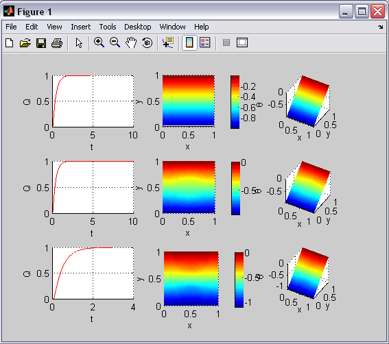
The m-file can now be saved as 'cp7.m' The following are several sample outputs from the code illustrating the ways to call the function with different types of return arguments.

>> cp7

icase =

     1


icase =

     2


icase =

     3

The entire matlab script can be seen below or downloaded here (right-click to save):

N = [30 30];
q = 1;
tend = 10.0;
movie_step = 10000000;

%case a)
icase =1
a1 = 1.;
a2 = 1.;
cp7_case(N,a1,a2,q,tend,movie_step,icase);

%case b)
icase =2
a1 = 1.;
a2 = 2.;
cp7_case(N,a1,a2,q,tend,movie_step,icase);

%case c)
icase =3
a1 = 1.;
a2 = 0.5;
cp7_case(N,a1,a2,q,tend,movie_step,icase);


%-----------------------------------------------------------------

%cp7_case

function cp7_case(N,a1,a2,q,tend,movie_step,icase)
T = zeros(N+1);
a = a1*ones(2*N+1);
a(1+2*N(1)/3:1+4*N(1)/3,1+2*N(2)/3:1+4*N(2)/3) = a2;
h = 1./N;
dt = min(min(h)^2/4/max([a1,a2]));
s=dt./h.^2;
x=linspace(0,1,N(1)+1);
y=linspace(0,1,N(2)+1);
it = 1;
time = [0:dt:tend];
Q = zeros(size(time));
for t = dt:dt:tend
    it = it +1;
    Told = T;
    T(2:N(1),2:N(2)) = Told(2:N(1),2:N(2))+...
               s(1)*(a(4:2:2*N(1),3:2:2*N(2)-1).*(Told(3:N(1)+1,2:N(2))-Told(2:N(1),2:N(2))) - a(2:2:2*N(1)-2,3:2:2*N(2)-1).*(Told(2:N(1),2:N(2))-Told(1:N(1)-1,2:N(2))))+...
               s(2)*(a(3:2:2*N(1)-1,4:2:2*N(2)).*(Told(2:N(1),3:N(2)+1)-Told(2:N(1),2:N(2))) - a(3:2:2*N(1)-1,2:2:2*N(2)-2).*(Told(2:N(1),2:N(2))-Told(2:N(1),1:N(2)-1)));   
    T(:,N(2)+1) = 0;         %BC top wall
    T(1,:) = T(2,:);         %BC left wall
    T(N(1)+1,:) = T(N(1),:); %BC right wall
    T(:,1) = T(:,2) - h(2)*q;
    heat_flux = (T(:,N(2)+1)-T(:,N(2)))/h(2);
    Q(it) = (heat_flux(1) + 2*sum(heat_flux(2:N(1))) + heat_flux(N(1)+1))*h(1)/2;
    if mod(t,dt*movie_step) == 0
        figure(2)
        surf(x,y,T')
        xlabel('x');
        ylabel('y');
        shading interp
        colormap jet
        set(gca,'DataAspectRatio',[1 1 1],'View',[0 90])
        colorbar('vert')
        figure(3)
        plot(time,Q,'r-')
        grid on
        pause(0.1)
    end
end
figure(1)
subplot(3,3,3*(icase-1)+1)
plot(time,Q,'r-')
grid on
xlabel('t')
ylabel('Q')
set(gca,'ylim',[0 1])
subplot(3,3,3*(icase-1)+2)
surf(x,y,T')
        xlabel('x');
        ylabel('y');
        shading interp
        colormap jet
        set(gca,'DataAspectRatio',[1 1 1],'View',[0 90])
        colorbar('vert')
subplot(3,3,3*icase)
surf(x,y,T')
        xlabel('x');
        ylabel('y');
        zlabel('\theta')
        shading interp
        colormap jet
        set(gca,'DataAspectRatio',[1 1 1],'View',[30 40],'ZLim',[min(T(:)) max(T(:))],'CLim',[min(T(:)) max(T(:))])