University of Colorado ::: Mechanical Engineering

CU Mechanical Engineering

Fluid Mechanics Matlab tutorials

Writing Matlab Functions: temperature distribution

In this example, we will write a function that computes the temperature distribution in a nuclear reactor fuel element.

We begin by declaring values for global use:

global n delta rspan options r T

In the beginning of this script, we define some of the variables we are going to use. The 'global' command defines global variables. Ordinarily, each MATLAB function, defined by an M-file, has its own local variables, which are separate from those of other functions, and from those of the base workspace. However, if several functions, and possibly the base workspace, all declare a particular name as global, they all share a single copy of that variable. Any assignment to that variable, in any function, is available to all the functions declaring it global.

The program essentially consists of the following block of code:

n = 100;
delta = 1.e-3;
rspan=linspace(delta,1,n+1);
options = odeset('RelTol',1e-12,'AbsTol',1e-12,'NormControl','on','MaxOrder',5);
T0=newton_mfile(@cp6_BV,2,1.e-10,0);
r=[0;r];  
T=[[T0,0];T]; 
[Tdirect,rdirect] = cp6_direct(n);
figure(1)
hold off
Texact= 9/32-r.^2/4-r.^4/32;
plot(r,Texact,'r-')
hold on
grid on
plot(r,T(:,1),'b:');
plot(rdirect,Tdirect,'g--');
legend('Exact','Shooting','Direct')

The linspace function generates linearly spaced vectors. It is similar to the colon operator ":", but gives direct control over the number of points. The odeset function lets you adjust the integration parameters of the ODE solvers. 'options = odeset('name1',value1,'name2',value2,...)' creates an options structure that you can pass as an argument to any of the ODE solvers. In the resulting structure, options, the named properties have the specified values. For example, 'name1' has the value 'value1'. Any unspecified properties have default values. The 'figure(1)' command tells matlab that the following commands are for a single plot. plot(X1,Y1,...) plots all lines defined by Xn versus Yn pairs. If only Xn or Yn is a matrix, the vector is plotted versus the rows or columns of the matrix, depending on whether the vector's row or column dimension matches the matrix.

The '@' symbol means that what follows is an embedded function. There are three different functions within this one that need to be considered. First, newton_mfile:

function x_root=newton_mfile(funhandle,x1,eps,reg)

To begin, all functions within matlab must begin by declaring that m-file is a function. This is accomplished by having the first line of the m-file having the word 'function' followed by the name of the variable that will be returned. This is consequently set equal to the name of the name of the file with the quantities that are passed to the function in parenthesis.

del = max([1.e-10,eps^2]);
x_guess(1) = [x1];
f_guess(1) = feval(funhandle,x_guess(1));
if abs(f_guess) < eps
   x_root=x_guess;
   disp('excellent guess');
   return
end

[y1, y2, ...] = feval(fhandle, x1, ..., xn) evaluates the function handle, fhandle, using arguments x1 through xn. If the function handle is bound to more than one built-in or M-file, (that is, it represents a set of overloaded functions), then the data type of the arguments x1 through xn determines which function is dispatched to.

The final step for this function goes as follows:

iter = 1;
check = logical(1);
tau=0.1;
while check
    iter = iter +1;
    x_guess(iter)=0;
    f_guess(iter)=0;
    f_h = feval(funhandle,x_guess(iter-1)+del);
    df=(f_h-f_guess(iter-1))/del;    
    dx(iter) = f_guess(iter-1)/df; 
    if iter >=  3
        tau=tau*dx(iter-1)/(dx(iter-1)-dx(iter));
    end
    if reg == 0
        x_guess(iter)=x_guess(iter-1)-dx(iter);
    else
        x_guess(iter)=x_guess(iter-1)-tau*dx(iter);
    end
    f_guess(iter) = feval(funhandle,x_guess(iter));
    if reg == 0 & abs(tau) < 1.0e-5 | abs(f_guess(iter)) < eps 
        x_root=x_guess(iter);
        check = logical(0);
    end
end

The following 'while' loop begins the iteration process to converge on a solution. The final condional 'if' statement is to ensure that iteratins stop when they converge.

The next function to consider is cp6_BV:

function f = cp6_BV(z)
global n delta rspan options r T
Tdelta  = z-1/4*delta^2-delta^4/32; 
dTdelta = -1/2*delta-delta^3/8;
[r,T] = ode15s(@rhs_cp6,rspan,[Tdelta dTdelta],options); 
f = T(end,1);

Again, all functions within matlab must begin by declaring that m-file is a function. We then define more global variables. The next lines define the boundary conditions with the out of pole corrections. A variable order solver based on the numerical differentiation formulas (NDFs), ode15s optionally uses the backward differentiation formulas, BDFs (also known as Gear's method). Like ode113, ode15s is a multistep solver. This is the entirety of this function.

Finally, we will look at cp6_direct:

function [T,r] = cp6_direct(N)

A = zeros(N+1);
S = zeros(N+1,1);
r = linspace(0,1,N+1)';
S(2:N) = -1 - r(2:N).^2/2;  
h = 1.0/N;
for i = 2:N 
    A(i,i-1) = 1/h^2-1/(2*h*r(i));
    A(i,i)   = -2/h^2;
    A(i,i+1) = 1/h^2+1/(2*h*r(i));
end
A(1,1:2) = [-1,1]; 
A(N+1,N+1) = 1;
T = inv(A)*S;

We start by declaring the function. The line 'S(2:N) = -1 - r(2:N).^2/2;' is the RHS of the equation. The for loop sets up the matrix. The first line after the for loop ends defines the boundary conditions. The last line sets up the solution.

The m-file can now be saved as 'cp6.m' The following are several sample outputs from the code illustrating the ways to call the function with different types of return arguments.

>> cp6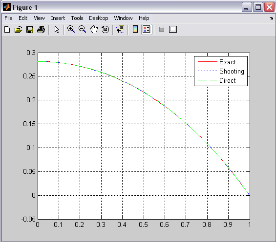

The entire matlab script can be seen below or downloaded here (right-click to save):

global n delta rspan options r T  
n = 100;
delta = 1.e-3;
rspan=linspace(delta,1,n+1);
options = odeset('RelTol',1e-12,'AbsTol',1e-12,'NormControl','on','MaxOrder',5);
T0=newton_mfile(@cp6_BV,2,1.e-10,0); 
r=[0;r];  
T=[[T0,0];T]; 
[Tdirect,rdirect] = cp6_direct(n);
figure(1)
hold off
Texact= 9/32-r.^2/4-r.^4/32;
plot(r,Texact,'r-')
hold on
grid on
plot(r,T(:,1),'b:');
plot(rdirect,Tdirect,'g--');
legend('Exact','Shooting','Direct')

%----------------------------------------------------

%newton_mfile

function x_root=newton_mfile(funhandle,x1,eps,reg)
del = max([1.e-10,eps^2]);
x_guess(1) = [x1];
f_guess(1) = feval(funhandle,x_guess(1));
if abs(f_guess) < eps
   x_root=x_guess;
   disp('excellent guess');
   return
end 
iter = 1;
check = logical(1);
tau=0.1;
while check
    iter = iter +1;
    x_guess(iter)=0;
    f_guess(iter)=0;
    f_h = feval(funhandle,x_guess(iter-1)+del);
    df=(f_h-f_guess(iter-1))/del;    
    dx(iter) = f_guess(iter-1)/df; 
    if iter >=  3
        tau=tau*dx(iter-1)/(dx(iter-1)-dx(iter));
    end
    if reg == 0
        x_guess(iter)=x_guess(iter-1)-dx(iter);
    else
        x_guess(iter)=x_guess(iter-1)-tau*dx(iter);
    end
    f_guess(iter) = feval(funhandle,x_guess(iter));
    if reg == 0 & abs(tau) < 1.0e-5 | abs(f_guess(iter)) < eps 
        x_root=x_guess(iter);
        check = logical(0);
    end
end
    
%-------------------------------------------------------

%cp6_BV

function f = cp6_BV(z)
global n delta rspan options r T
Tdelta  = z-1/4*delta^2-delta^4/32; 
dTdelta = -1/2*delta-delta^3/8;
[r,T] = ode15s(@rhs_cp6,rspan,[Tdelta dTdelta],options); 
f = T(end,1);  
%------------------------------------------------------------

%cp6_direct

function [T,r] = cp6_direct(N)

A = zeros(N+1);
S = zeros(N+1,1);
r = linspace(0,1,N+1)';
S(2:N) = -1 - r(2:N).^2/2;  
h = 1.0/N;
for i = 2:N 
    A(i,i-1) = 1/h^2-1/(2*h*r(i));
    A(i,i)   = -2/h^2;
    A(i,i+1) = 1/h^2+1/(2*h*r(i));
end
A(1,1:2) = [-1,1]; 
A(N+1,N+1) = 1;
T = inv(A)*S;