CU Mechanical EngineeringFluid Mechanics Matlab tutorials |
Writing Matlab Functions: ice build-up
In this example, we will write a function that computes the amount ice build-up (on a lake, for example).
To begin, we label the global values of the script:
global L
In the beginning of this script, we define some of the variables we are going to use. The 'global' command defines global variables. Ordinarily, each MATLAB function, defined by an M-file, has its own local variables, which are separate from those of other functions, and from those of the base workspace. However, if several functions, and possibly the base workspace, all declare a particular name as global, they all share a single copy of that variable. Any assignment to that variable, in any function, is available to all the functions declaring it global.
The rest of the script is as follows:
L = 0.5;
tspan=[0:0.1:10];
options = odeset('RelTol',1e-12,'AbsTol',1e-6,'NormControl',...
    'on','MaxOrder',2);
[T,Y] = ode15s(@fun_cp5,tspan,[0.01 0.5],options);
figure(1)
hold off
plot(T,Y(:,1:2))
grid on
legend('h','h_t',2);
title('Ice Build-Up');
xlabel('t');
ylabel('h, h_t');
The time interval for the set is defined in a vector. The odeset function lets you adjust the integration parameters of the ODE solvers. 'options = odeset('name1',value1,'name2',value2,...)' creates an options structure that you can pass as an argument to any of the ODE solvers. In the resulting structure, options, the named properties have the specified values. For example, 'name1' has the value 'value1'. Any unspecified properties have default values. A variable order solver based on the numerical differentiation formulas (NDFs), ode15s optionally uses the backward differentiation formulas, BDFs (also known as Gear's method). Like ode113, ode15s is a multistep solver. The 'figure(1)' command tells matlab that the following commands are for a single plot.
It should be noted that the '@' sign means right before 'fun_cp5' means that 'fun_cp5' is a function, not a variable. We'll define the fun_cp5 function as follows:
function dy = fun_cp5(t,y)
To begin, all functions within matlab must begin by declaring that m-file is a function. This is accomplished by having the first line of the m-file having the word 'function' followed by the name of the variable that will be returned. This is consequently set equal to the name of the name of the file with the quantities that are passed to the function in parenthesis.
The rest of the function goes as follows:
global L;
dy = zeros(2,1);
dy(1) = y(2);
dy(2) = -(2*y(2)^2+4*L*(1+y(1))/(2+y(1))*y(2)-4*L/(2+y(1)))/y(1)^2;
Here we again define global variables and we define the differential equations we will use to compute the amount of ice build-up.
The m-file can now be saved as 'cp5.m' The following are several sample outputs from the code illustrating the ways to call the function with different types of return arguments.
>> cp5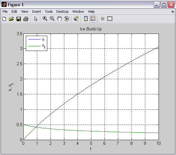
The entire matlab script can be seen below or downloaded here (right-click to save):
global L
L = 0.5;
tspan=[0:0.1:10];
options = odeset('RelTol',1e-12,'AbsTol',1e-6,'NormControl',...
    'on','MaxOrder',2);
[T,Y] = ode15s(@fun_cp5,tspan,[0.01 0.5],options);
figure(1)
hold off
plot(T,Y(:,1:2))
grid on
legend('h','h_t',2);
title('Ice Build-Up');
xlabel('t');
ylabel('h, h_t');

%------------------------------------------------

%fun_cp5

function dy = fun_cp5(t,y)
global L;
dy = zeros(2,1);
dy(1) = y(2);
dy(2) = -(2*y(2)^2+4*L*(1+y(1))/(2+y(1))*y(2)-4*L/(2+y(1)))/y(1)^2;