CU Mechanical EngineeringFluid Mechanics Matlab tutorials |
Writing Matlab Functions: fluid draining from a spherical tank
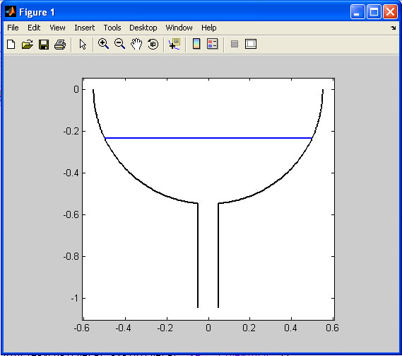
The power of using Matlab functions will once again be explored with an example which solves for fluid draining from a spherical tank by means of a cylindrical pipe. This example also takes advantage of some of the basic graphics capabilities which exist within Matlab and plots the fluid level as the tank empties in real time.
To begin, all functions within matlab must begin by declaring that m-file is a function. This is accomplished by having the first line of the m-file having the word 'function' followed by the name of the variable which will be returned. This is consequently set equal to the name of the name of the file with the quantities that are passed to the function in parenthesis. For this excersize, we will begin by calling a function with the dependant variables of h,D,d and H which represent the initial height of the fluid, the diameter of the speherical tank, the diameter of the draining pipe and the length of the draining pipe repectively. Since this function does not return any values, we begin the funciton m-file as follows:
function drain(h,D,d,H)
To begin the function, the first step is to identify all the constants and variables which will be needed within the function. Since these variables must be defined before they can be used within the function, it logically makes the most sense to call them at the beginning after the initial function declaration. Another note to remember is that any text or code following a percent sign is considered a comment and is not executed by matlab. This is a convenient way to document m-files for later reference.
time_stretch=10; % how much slower is plotign time vs. real time
g=9.81; %acceleration of gravity
R=D/2;
r=d/2;
theta0=asin(d/D);
h0=R*sin(-pi/2+theta0); % height where pipe connects to the speherical tank
r0=R*cos(-pi/2+theta0); % radius where pipe connects to the speherical tank
Ntheta=100;
dtheta=(pi/2-theta0)/Ntheta;
Next, the hold command is utilized for the purpose of plotting the fluid level as it drains from the tank. From the Matlab help (which can be called at any point from the command line by typing 'help' followed by the topic), we can find out that "HOLD ON holds the current plot and all axis properties so that subsequent graphing commands add to the existing graph. HOLD OFF returns to the default mode whereby PLOT commands erase the previous plots and reset all axis properties before drawing new plots." The following commands are used to plot the tank and drain.
hold off
plot(R*cos(theta),R*sin(theta),'k-','LineWidth',2);
hold on
plot(-R*cos(theta),R*sin(theta),'k-','LineWidth',2);
plot([r0,r0],[h0,-R-H],'k-','LineWidth',2);
plot(-[r0,r0],[h0,-R-H],'k-','LineWidth',2);
The plot is then centered by adjusting the access by using the 'set' command to alter the axis of the plot.
set(gca,'Xlim',[-R*1.1,R*1.1],'Ylim',[-R*1.1-H,0.1*R])
set(gca,'PlotBoxAspectRatio',[1.1*D 1.2*R+H 1.1*D])
Next, several parameters are defined in order to plot the fluid. The 'y' coordinate is defined in terms of the radius of the tank and height of the fluid and the discrete step variables are defined.
y=-R+h;
delh=0.01*R;
dt=0.001;
h1=plot([-radius(y),radius(y)],[y,y],'b-','LineWidth',2);
set(h1,'EraseMode','normal')
The last step is to set up a loop to invoke the ODE solver while there is still fluid in the system. For this purpose, a 'while' loop is used. This loop executes until the test condition is not true - in this case it means that as long as there is fluid in the system, the loop will execute. After the solver returns the result, the figure is updated and then a pause is used to simulate real-time draining. This loop is written as:
while y > -R-H
   % Call the ODE solver ode15s.
   dt=abs(delh/dh(0,y));
   [time,Y] = ode15s(@dh,[0,dt],y);
   y=Y(end);
   set(h1,'XData',[-radius(y),radius(y)],'YData',[y,y])
   pause(time_stretch*dt);
end
It is important to note that in order to use any of the ODE solvers, one of the arguments must be a function. In this examble, the function name is 'dh'. To indicate that this is a function and not a variable, matlab requires that the name of the function be preceeded by the '@' character.
Since the 'dh' function does not exist, we have to create it. This function can be a separate m-file such as this function or we can use what are known as 'nested functions'. These functions act just as other functions but only work within the primary function. The function begins with the same function declaration as a normal function, but this cannot be referenced from the command line or other functions. Since the additional two functions necessary for the 'drain' function are only needed for this function, this will be fine.
The first function we will write is the 'dh' function which is passed to the ODE solver. This function returns the rate of change for the surface of the liquid.
   function dydt = dh(t,y)
       if y>=h0 %the radius of the surface of the fluid is R^2-h^2
          dydt = -sqrt(2*g*(R+y+H))*radius(y)^2/r^2;
       elseif -R-H < y & y < h0 % no fluid s left in spherical tank,
                                  the fluid is draining out of the pipe
          dydt = -sqrt(2*g*(R+y+H))*radius(y)^2/r^2;
       else % the fluid is drained out completely
          dydt = 0;
       end
   end
The second nested function returns the radius of the fluid given the height of the liquid. This has two parts, one if the level of the liquid is still in the sphere and the second if the fluid level is within the draining cylinder.
   function r0 = radius(y)
       if y>=h0 %the radius of the surface of the fluid is R^2-h^2
          r0 = sqrt(R^2-y^2);
       elseif -R-H < y & y < h0 % no fluid s left in spherical tank,
                                  the fluid is draining out of the pipe
          r0 = r;
       else % the fluid is drained out completely
          r0 = 0;
       end
   end
The function can now be saved as 'drain.m' and can be executed from the Matlab command prompt.
The entire matlab script can be seen below or downloaded here (right-click to save):
% h - iniital height of the fluid
% D - diameter of the spherical tank
% d - diameter of the draiing pipe
% H - lenght of the draining pipe
function drain(h,D,d,H)

time_stretch=10; % how much slower is plotign time vs. real time
g=9.81; %acceleration of gravity
R=D/2;
r=d/2;
theta0=asin(d/D);
h0=R*sin(-pi/2+theta0); % height where pipe connects to the speherical tank
r0=R*cos(-pi/2+theta0); % radius where pipe connects to the speherical tank
Ntheta=100;
dtheta=(pi/2-theta0)/Ntheta;
theta=[-pi:dtheta:-pi/2-theta0];
hold off
plot(R*cos(theta),R*sin(theta),'k-','LineWidth',2);
hold on
plot(-R*cos(theta),R*sin(theta),'k-','LineWidth',2);
plot([r0,r0],[h0,-R-H],'k-','LineWidth',2);
plot(-[r0,r0],[h0,-R-H],'k-','LineWidth',2);
set(gca,'Xlim',[-R*1.1,R*1.1],'Ylim',[-R*1.1-H,0.1*R])
set(gca,'PlotBoxAspectRatio',[1.1*D 1.2*R+H 1.1*D])

y=-R+h;
delh=0.01*R;
dt=0.001;
h1=plot([-radius(y),radius(y)],[y,y],'b-','LineWidth',2);
set(h1,'EraseMode','normal')

%plots real time

while y > -R-H
   % Call the ODE solver ode15s.
   dt=abs(delh/dh(0,y));
   [time,Y] = ode15s(@dh,[0,dt],y);
   y=Y(end);
   set(h1,'XData',[-radius(y),radius(y)],'YData',[y,y])
   pause(time_stretch*dt);
end
   %Define the ODE function as nested function, h - height of the fluid
   function dydt = dh(t,y)
       if y>=h0 %the radius of the surface of the fluid is R^2-h^2
          dydt = -sqrt(2*g*(R+y+H))*radius(y)^2/r^2;
       elseif -R-H < y & y < h0 % no fluid s left in spherical tank,
                                  the fluid is draining out of the pipe
          dydt = -sqrt(2*g*(R+y+H))*radius(y)^2/r^2;
       else % the fluid is drained out completely
          dydt = 0;
       end
   end
   function r0 = radius(y)
       if y>=h0 %the radius of the surface of the fluid is R^2-h^2
          r0 = sqrt(R^2-y^2);
       elseif -R-H < y & y < h0 % no fluid s left in spherical tank,
                                  the fluid is draining out of the pipe
          r0 = r;
       else % the fluid is drained out completely
          r0 = 0;
       end
   end
end