CU Mechanical EngineeringDynamics Matlab tutorials |
Writing Matlab Functions: damped spring system
In this example, we will create a Simulink model for a mass attatched to a spring with a linear damping force.
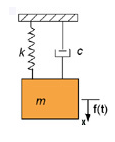
A mass on a spring with a velocity-dependant damping force and a time-dependant force acting upon it will behave according to the following equation:
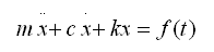
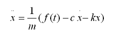
The model will be formed around this equations. In this equation, 'm' is the equivalent mass of the system; 'c' is the damping constant; and 'k' is the constant for the stiffness of the spring. First we want to rearrange the above equation so that it is in terms of acceleration; then we will integrate to get the expressions for velocity and position. Rearranging the equation to accomplish this, we get:
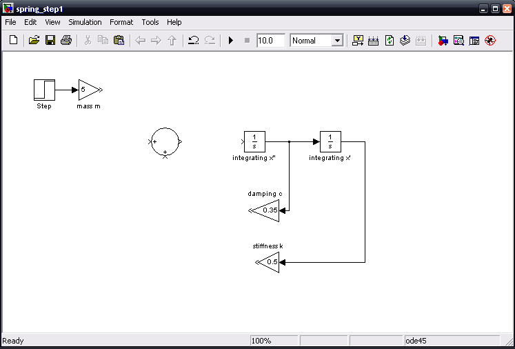
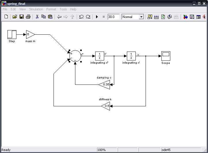
To build the model, we start with a 'step' block and a 'gain' block. The gain block represents the mass, chich we will se equal to 5. We also know that we will need to integrate twice, that we will need to add these equations together, and that there are two more constants to consider. The damping constant 'c' will act on the velocity, that is, after the first integration, and the constant 'k' will act on the position, or after the second integration. Let c = 0.35 and let k = 0.5. Laying all these block out to get an idea of how to put them together, we get:
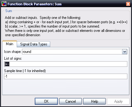
By looking at the equation in terms of acceleration, it is clear that the damping term and spring term are summed negatively, while the mass term is still positive. To add places and change signs of terms being summed, double-click on the sum function block and edit the list of signs:
Once we have added places and corrected the signs for the sum block, we need only connect the lines to their appropriate places. To be able to see what is happening with this spring system, we add a 'scope' block and add it as follows:
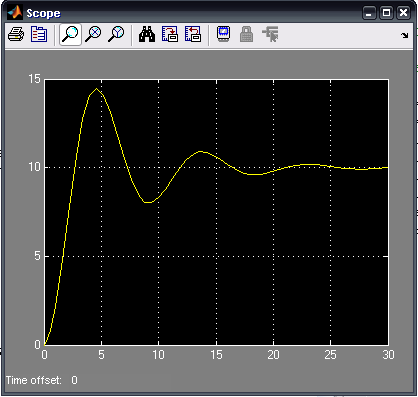
The values of 'm', 'c' and 'k' can be altered to test cases of under-damping, critical-damping and over-damping. To accurately use the scope, right-click the graph and select "Autoscale".
The mdl-file can now be saved. The following is a sample output when the model is run for 30 iterations.
The entire model can be downloaded here (right-click to save):