CU Mechanical EngineeringDynamics Matlab tutorials |
Writing Matlab Functions: bouncing ball model
In this example, we will create a Simulink model for the position and velocity of a bouncing ball.
A ball falling under gravity will obey the following equations of motion:
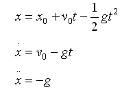
The model will be formed around these equations. We will start with gravitational acceleration, then intergrate once to obtain an expression for velocity, and once more to find an expression for position. This first step will look something like this:
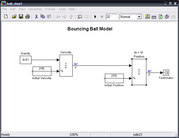
Here we input the gravitational constant, -9.81 and the initial velocity into an integrator block to get our expression for velocity. This expression is fed into another integrator block along with the initial position, giving us an expression for position. The 'Terminator' block is used to 'terminate' output signals, which prevents warnings about unconnected output ports.
Next, we need to modify the position block further. We want it to ensure that the ball never goes through the floor; that is, that the position is always positive. We also want it to reset and re-evaluate each time the ball bounces. To do this, we make the following adjustments:
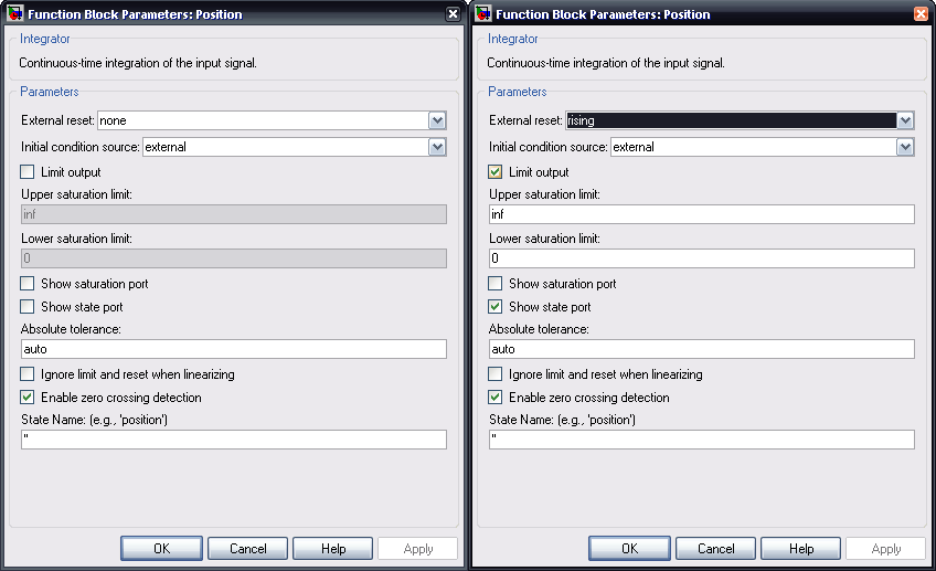
Double-clicking the position block should produce a menu that looks like the above menu on the left. We want to add an external reset which is rising, limit the output, and show the state port. Once we've done this, we can add the following blocks:
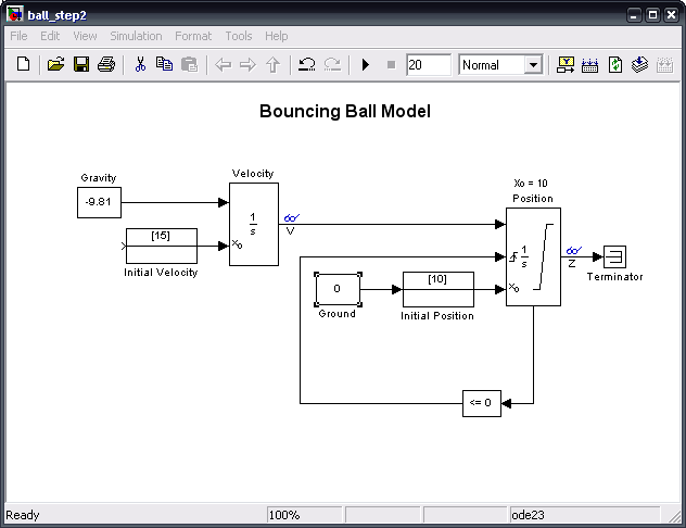
We add a zero input, called ground, since each bounce after the first will have an initial position of 0. The loop at the bottom verifies that the function does not go below zero and resets the position block after each bounce. Now all that must be modified is the velocity block. We change it in much the same way we changed the position block; we want to add an external reset which is rising, and we want to show the state port. It is not necessary to limit the output this time. Once we have done this, we can add the final blocks:
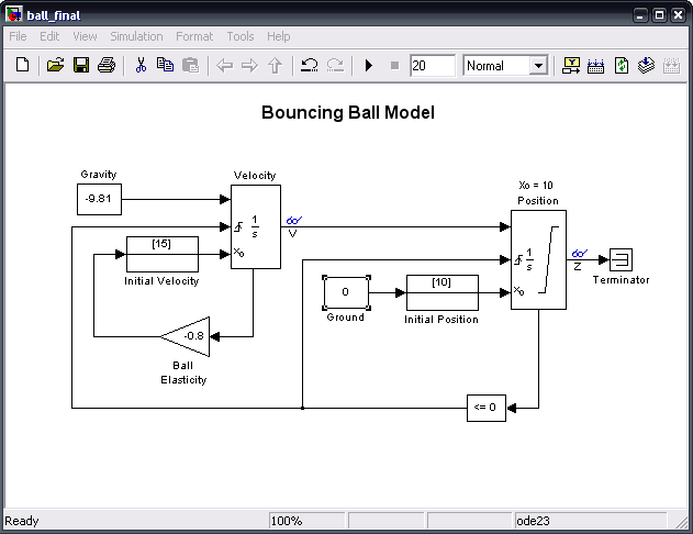
The bottom line that feeds to the middle port of the velocity block resets that block as well each time the ball hits the ground. For this problem, we include a ball elasticity of -0.8 to account for loss of energy due to air resistance and internal forces.
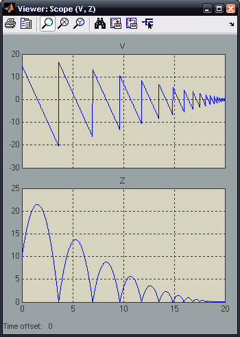
The mdl-file can now be saved. The following is a sample output when the model is run for 20 iterations. The window on the top is the velocity and the window on the bottom plots position.
The entire model can be downloaded here (right-click to save):