CU Mechanical EngineeringDynamics Matlab tutorials |
Writing Matlab Functions: the inverted pendulum
In this example, we will create a Simulink model for an inverted pendulum on a cart.
In this example, we will implement a PID controller which can only be applied to a single-input-single-output (SISO) system,so we will be only interested in the control of the pendulums angle. Therefore, none of the design criteria deal with the cart's position. We will assume that the system starts at equilibrium, and experiences an impulse force of 1 newton. The pendulum should return to its upright position within 5 seconds, and never move more than 0.05 radians away from the vertical.
This system is tricky to model in Simulink because of the physical constraint (the pin joint) between the cart and pendulum which reduces the degrees of freedom in the system. Both the cart and the pendulum have one degree of freedom (X and theta, respectively). We will then model Newton's equation for these two degrees of freedom.
It is necessary, however, to include the interaction forces N and P between the cart and the pendulum in order to model the dynamics. The inclusion of these forces requires modeling the x and y dynamics of the pendulum in addition to its theta dynamics. Generally, we would like to exploit the modeling power of Simulink and let the simulation take care of the algebra. Therefore, we will model the additional x and y equations for the pendulum.
However, xp and yp are exact functions of theta. Therefore, we can represent their derivatives in terms of the derivatives of theta.
These expressions can then be substituted into the expressions for N and P. Rather than continuing with algebra here, we will simply represent these equations in Simulink. Simulink can work directly with nonlinear equations, so it is unnecessary to linearize these equations.
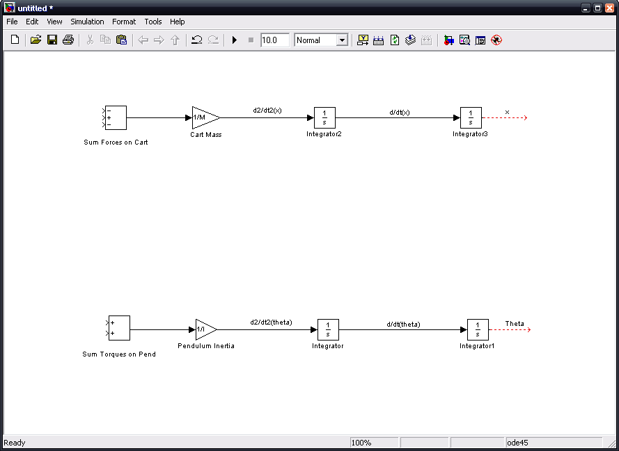
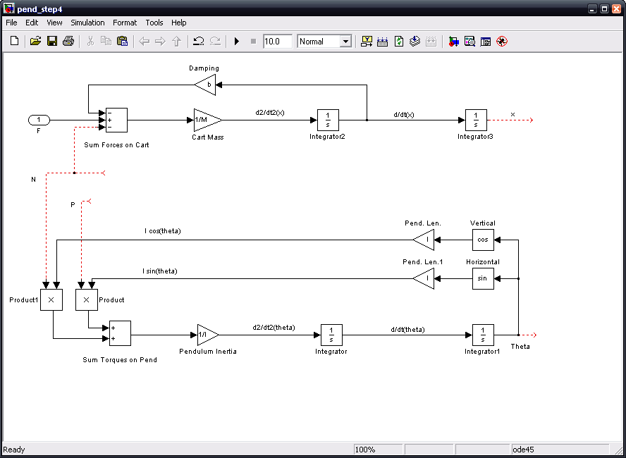
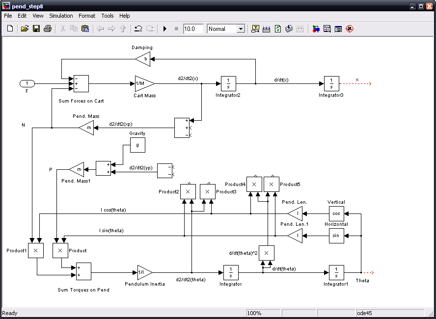
This is a large model and will take a lot of space, so give yourself pleny of room to work with. It would also be a good idea to label each line and box to avoid confusion later. To begin, start with a summation block for the forces on the cart. Below it, do the same for the torques on the pendulum. These two lines will mimick each other at first. For each, connect the sum box to a gain box, then an integrator box, and then connect this to another integrator box. For the cart, modify the gain box so that the gain is 1/M. Modify the gain for the pendulum to be 1/I. It may be worth labeling each line as the equation it represents (see the diagram below):
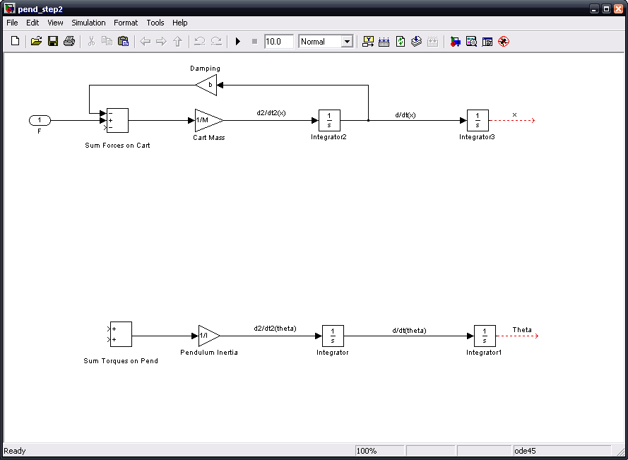
Next we will add two forces acting on the cart. Add a gain block to represent damping and label it as such. Change the value to 'b'. Tap a line off the d/dt(x) line, since damping is velocity dependant, and connect it to the 'damping' gain block. Now connect this block to the topmost port on the sum block so that the damping force is negative. Now add an input block and label it F. Connect it to the middle, positive port on the sum.
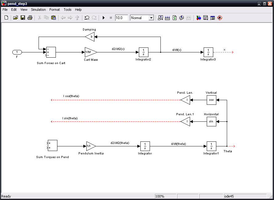
Now, we will apply the forces N and P to both the cart and the pendulum. We need to construct the components of these forces, 'N L cos(thenta)' and 'P L sin(theta). Add two 'trigonometric function' blocks. Make one of them a cosine block and leave the other as sine. Arrange these so that the cosine block is above the sine block which is above the last integrator block for your theta function. Tap a line from the theta line and connect it to both the sine and cosine blocks. Label the cos block as "Vertical" and the sin block as "Horizontal", these being the force components they represent. Connect a new gain block to the sine block and another to the cosine block. These gain blocks will be identical. Call this block 'Pend. Len.' and make its value 'l' (lowercase L). Finally, extend a line from each gain block. Label the top line "l cos(theta)" and the bottom line "l sin(theta)".
Now that the pendulum components are available, we can apply the forces N and P. We will assume we can generate these forces, and just draw them coming from nowhere for now. Add two product blocks next to each other to the left and above the Sum Torques block. These will be used to multiply the forces N and P by their appropriate components. Rotate them to face downward. Connect the right product block to the upper input on the Sum Torques block and the left product lock to the lower input. Connect the "l sin(theta)" line to the right inuput of the right product block, and the "l cos(theta)" line to the right input of the left product block. Now create a line that leads to the left input of the right product block; label this line 'P'. Create another line leading to the left input of the left block and label this line 'N'. Finally, tap a line off of 'N' and connect it to the bottom input of the Sum Forces block.
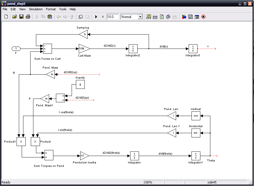
Next, we will represent the force N and P in terms of the pendulum's horizontal and vertical accelerations from Newton's laws. Insert two identical gain blocks labeled "Pend. Mass" and with value 'm'. Connect one to the opening on line P and the other to the opening on N. Connect a line to the top Pend. mass and label it "d2/dt2(xp)". Add a sum block and connect it to the lower Pend. mass block; leave both inputs positive. Insert a constant; give it a value of 'g' and label it gravity, then connect it to the top input of the sum block. Extend a line out from the bottom input of the sum block and label that line d2/dt2(yp).
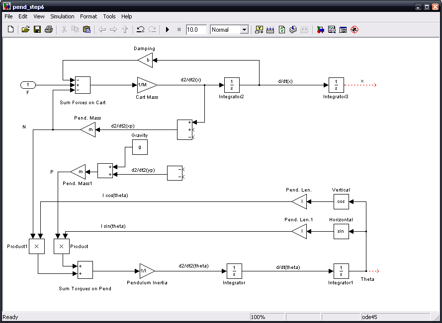
Now, we will begin to produce the signals which contribute to d2/dt2(xp) and d2/dt2(yp). Insert a Sum block to the right of the d2/dt2(yp) open end. Change the Sum block's signs to "--" to represent the two terms contributing to d2/dt2(yp). Flip the Sum block left-to-right and connect it's output to the d2/dt2(yp) signal. Insert a Sum block to the right of the d2/dt2(xp) open end. Change the Sum block's signs to "++-" to represent the three terms contributing to d2/dt2(xp). Flip the Sum block left-to-right and connect it's output to the d2/dt2(xp) signal. The first term of d2/dx2(xp) is d2/dx2(x). Tap a line off the d2/dx2(x) signal and connect it to the topmost (positive) input of the newest Sum block.
Now, we will generate the terms d2/dt2(theta)*lsin(theta) and d2/dt2(theta)*lcos(theta). Insert two Product blocks next to each other to the right and below the Sum block associated with d2/dt2(yp). Rotate the left Product block 90 degrees. Flip the other product block left-to-right and also rotate it 90 degrees. Tap a line off the l sin(theta) signal and connect it to the left input of the left Product block. Tap a line off the l cos(theta) signal and connect it to the right input of the right Product block. Tap a line off the d2/dt2(theta) signal and connect it to the right input of the left Product block. Tap a line of this new line and connect it to the left input of the right Product block.
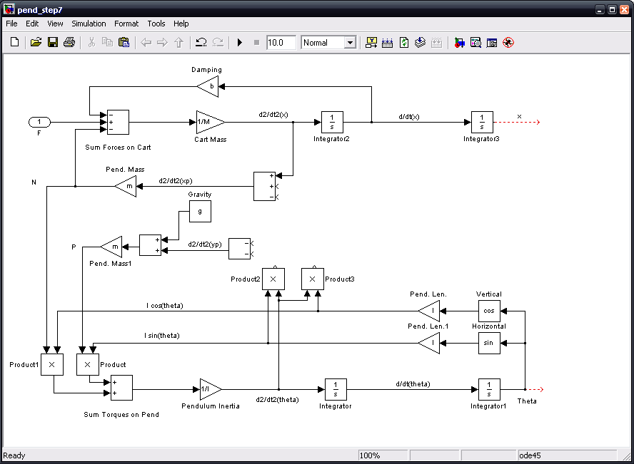
Now, we will generate the terms (d/dt(theta))^2*lsin(theta) and (d/dt(theta))^2*lcos(theta). Insert two Product blocks next to each other to the right and slightly above the previous pair of Product blocks. Rotate the left Product block 90 degrees. Flip the other product block left-to-right and also rotate it 90 degrees. Tap a line off the l cos(theta) signal and connect it to the left input of the left Product block. Tap a line off the l sin(theta) signal and connect it to the right input of the right Product block. Insert a third Product block and insert it slightly above the d/dt(theta) line. Label this block "d/dt(theta)^2". Tap a line off the d/dt(theta) signal and connect it to the left input of the lower Product block. Tap a line of this new line and connect it to the right input of the lower Product block. Connect the output of the lower Product block to the free input of the right upper Product block. Tap a line of this new line and connect it to the free input of the left upper Product block.
Finally, we will connect these signals to produce the pendulum acceleration signals. In addition, we will create the system outputs x and theta. Connect the d2/dt2(theta)*lsin(theta) Product block's output to the lower (negative) input of the d2/dt2(yp) Sum block. Connect the d2/dt2(theta)*lcos(theta) Product block's output to the lower (negative) input of the d2/dt2(xp) Sum block. Connect the d/dt(theta)^2*lcos(theta) Product block's output to the upper (negative) input of the d2/dt2(yp) Sum block. Connect the d/dt(theta)^2*lsin(theta) Product block's output to the middle (positive) input of the d2/dt2(xp) Sum block. Insert an Out block attached to the theta signal. Label this block "Theta". Insert an Out block attached to the x signal. Label this block "x". It should automatically be numbered 2.
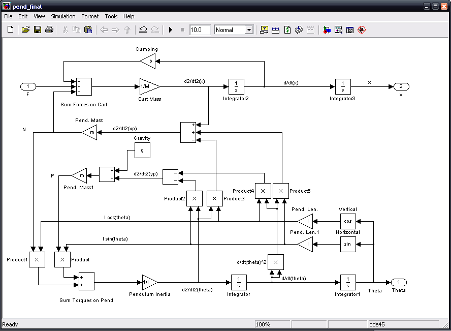
The mdl-file can now be saved. The entire model can be downloaded here (right-click to save):
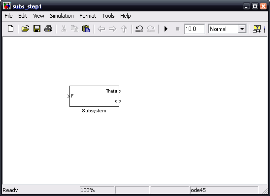
We now want to take this model we just created and make it a subsystem of another model. To do this, create a new window and insert a subsystem block. Open the subsystem block and drag the entire model we just built into it. Label the subsystem "Inverted Pendulum".
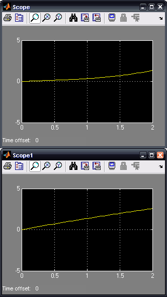
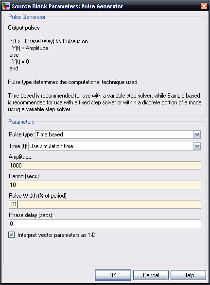
Now, we will apply a unit impulse force input, and view the pendulum angle and cart position. An impulse can not be exactly simulated, since it is an infinite signal for an infinitesimal time with time integral equal to 1. Instead, we will use a pulse generator to generate a large but finite pulse for a small but finite time. The magnitude of the pulse times the length of the pulse will equal 1. Insert a Pulse Generator block and two scope blocks. Connect the pulse generator to the F input and connect the Theta and x outputs each to a scope.
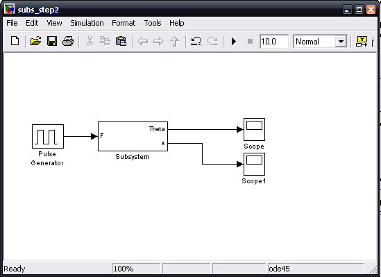
Edit the pulse generator so that the period value is "10" (a long time between a chain of impulses - we will be interested in only the first pulse); change the Pulse width value to ".01" (meaning .01% of 10 seconds, or .001 seconds); Change the amplitude to 1000 (1000 times .001 is 1, providing a unit impulse); now close the dialogue.
Now we must set an appropriate simulation time to view the response. Select Configuration Parameters from the simulation menu and change the stop time value to 2 seconds. Before running this, it is necessary to set the physical constants we are using. Enter the following commands into the Matlab prompt:
M = 0.5;
m = 0.2;
b = 0.1;
i = 0.006;
g = 9.81;
l = 0.3
Below is a sample response for this model.