Writing Matlab Functions: the Henon map

In this example, we will write a function that plots a Henon map and compares the shapes of curves starting at different initial values.

Consider the Henon map described by

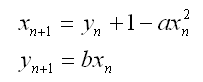
We want Matlab to generate plots for this map starting with a couple distinct initial values to compare the shapes of the curves. First, we let a = 1.4 and b = 0.3. We will have Matleb plot the first 10,000 points of the form (xn,yn) with the initial values x0 = 0 and y0 = 0. To begin, all functions within matlab must begin by declaring that m-file is a function. This is accomplished by having the first line of the m-file having the word 'function' followed by the name of the variable that will be returned. This is consequently set equal to the name of the name of the file with the quantities that are passed to the function in parenthesis. For the purpose of this exercise, the name of the function will be 'henon' and the first line of the function is as follows:

function henon

x(1) = 0;
y(1) = 0;

for i = 2:10000
    x(i) = y(i-1)+1-1.4*(x(i-1)^2);
    y(i) = 0.3*x(i-1);
    x(i) = keepx(x(i));
    y(i) = keepy(y(i));
end

After neming the function, we state our initial conditions: x=y=0. The 'for' loop tells us that it will evaluate the first 10,000 terms. The first two lines of the 'for' loop are the equations for the Henon map. The following two lines reference two other equations we will need to specify where we plot out points and the boundary of the plot. The area of the plot we are interested in is when x is between -1.5 and 1.5, and when y is between -0.45 and 0.45, so we will have our function discard all points that fall outside this region.

function res = keepx(in)

if in > 1.5
    res = 0;
elseif in < -1.5
    res = 0;
else
    res = in;
end

This simple function keeps the x points mapped to the region of interest. The conditional 'if' statement says that each point of the function of x greater than 1.5 gets mapped to zero; so do all points when x is less than -1.5. For all other x, the function remains unchanged.

We now do the same thing for the y-coordiantes:

function res = keepy(in)

if in > 0.45
    res = 0;
elseif in < -0.45
    res = 0;
else
    res = in;
end

This simple function keeps the y points mapped to the region of interest the exact same way the keepx function kept the x points. Before we copnsider any other initiaql conditions, we need to look at the plot. To plot the results in a two-dimensional plot, we add a 'plot' command after the first function. Since the plot is a function of x and y, it cannot follow the second or third functions but must follow the first, like so:

function henon

x(1) = 0;
y(1) = 0;

for i = 2:10000
    x(i) = y(i-1)+1-1.4*(x(i-1)^2);
    y(i) = 0.3*x(i-1);
    x(i) = keepx(x(i));
    y(i) = keepy(y(i));
end

plot(x,y)

Now choose as initial coordinates x0 = 0.63135448, y0 = 0.18940634. Simply change the x(0) and y(0) definitiions at the beginning of the function, and then save before evaluating:

function henon

x(1) = 0.63135448;
y(1) = 0.18940634;

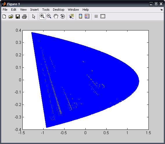
Evaluating this with both sets of initial conditions seems to indicate that the shape of the curve is independant of initial conditions.

The m-file can now be saved. The following are several sample outputs from the code illustrating the ways to call the function with different types of return arguments.

>> henon

The entire matlab script can be seen below or downloaded here (right-click to save):

function henon

x(1) = 0.63135448;
y(1) = 0.18940634;

for i = 2:10000
    x(i) = y(i-1)+1-1.4*(x(i-1)^2);
    y(i) = 0.3*x(i-1);
    x(i) = keepx(x(i));
    y(i) = keepy(y(i));
end

plot(x,y)

function res = keepx(in)

if in > 1.5
    res = 0;
elseif in < -1.5
    res = 0;
else
    res = in;
end

function res = keepy(in)

if in > 0.45
    res = 0;
elseif in < -0.45
    res = 0;
else
    res = in;
end