CU Mechanical Engineering Dynamics Matlab tutorials

---

Writing Matlab Functions: bouncing ball problem

In this example, we will write a function that maps the motion of a ball bouncing on a sinusoidally oscillating floor.

The motion of a bouncing ball, on successive bounces, when the floor oscillates sinusoidally can be described by the Chirikov map:

We want Matlab to create two-dimensional maps for different values of K and the stated values of p and q. To do this, we need to define two functions: one that includes the above equations, and another to keep it in the boundaries also defined above. To begin, all functions within matlab must begin by declaring that m-file is a function. This is accomplished by having the first line of the m-file having the word 'function' followed by the name of the variable that will be returned. This is consequently set equal to the name of the name of the file with the quantities that are passed to the function in parenthesis. For the purpose of this exercise, the name of the function will be 'bouncy' and the first line of the function is as follows:

function bouncy

p(1) = 1;
q(1) = 1;
K = 0.8;
for i = 2:5000
    p(i) = p(i-1)-K*sin(q(i-1));
    q(i) = q(i-1)+p(i);
    p(i) = periodic(p(i));
    q(i) = periodic(q(i));
end

After defining 'bouncy' as a function, we say that the iterating equations will start with p=q=1, and our initial K value is 0.8. The 'for' loop begins by stating that we will be looking at the first five-thousand iteraions. The next two lines define the two iterative equations we are given for the problem. The following two lines let us keep this function periodic, so long as we define the periodic function. This we will do now.

function res = periodic(in)

if in > pi
    res = in - 2*pi;
elseif in < -pi
    res = in + 2*pi;
else
    res = in;
end

This is the entirety of the periodic function. The condiitional 'if' statements insure that when any function increases beyond pi, 2pi is subtracted from the function; also, if it decreases beyond negative pi, 2pi is added to the function. In all other cases, the function keeps its original value.

To plot the results in a two-dimensional plot, we add a 'plot' command after the first function. Since the plot is a function of p and q, it cannot follow the second function but must follow the first, like so:

function bouncy

p(1) = 1;
q(1) = 1;
K = 0.8;
for i = 2:5000
    p(i) = p(i-1)-K*sin(q(i-1));
    q(i) = q(i-1)+p(i);
    p(i) = periodic(p(i));
    q(i) = periodic(q(i));
end

plot (p,q)

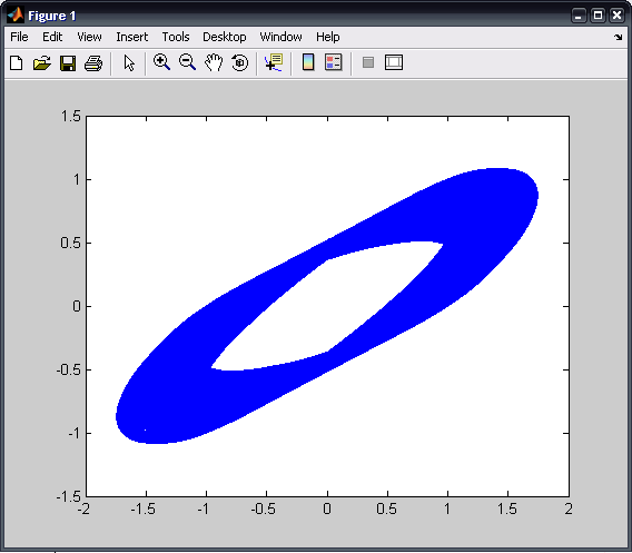
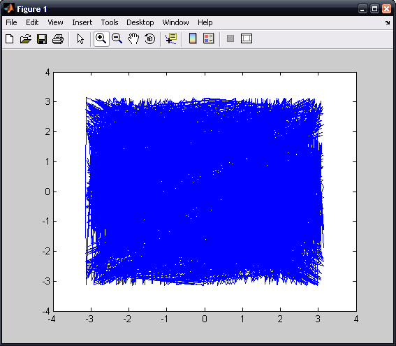
The function can now be evaluated for various values of K; we will look at the plots for K = 0.8, 3.2 and 6.4, in that order. Be sure to save the .m file each time you chance the value of K.

The m-file can now be saved. The following are several sample outputs from the code illustrating the ways to call the function with different types of return arguments.

>> bouncy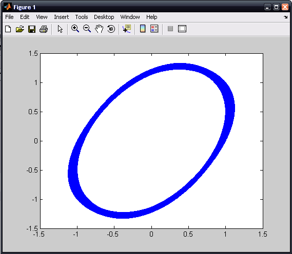

The entire matlab script can be seen below or downloaded here (right-click to save):

function bouncy

p(1) = 1;
q(1) = 1;
K = 6.4;
for i = 2:5000
    p(i) = p(i-1)-K*sin(q(i-1));
    q(i) = q(i-1)+p(i);
    p(i) = periodic(p(i));
    q(i) = periodic(q(i));
end

plot (p,q)

function res = periodic(in)

if in > pi
    res = in - 2*pi;
elseif in < -pi
    res = in + 2*pi;
else
    res = in;
end

---